September 2026
Code: GitHub repository · Training and evaluation · Downstream results
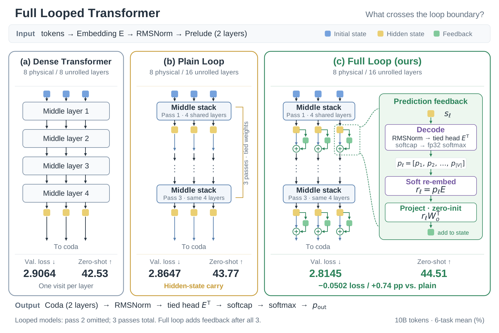
In a looped (weight-tied, middle-cycle) transformer, we include the LM head and the tied embedding inside the loop: at every loop junction, decode the current state into a full next-token distribution, softly re-embed it with the tied embedding matrix, and add a zero-initialized projection of this "draft prediction" back to the residual stream. On a controlled 57M/10B-token A/B testbed this is worth −0.050 validation loss over the plain loop (6.4× the cross-seed noise floor) and +0.74 mean zero-shot accuracy, and the 57M looped model overtakes a 113M dense model of the same unrolled depth on the downstream mean. A replacement variant — carrying only the re-embedded prediction between iterations — destroys the model, locating the value precisely: the prediction is a powerful auxiliary signal, not a substitute for the latent state.
A looped transformer applies a shared middle stack $L$ times between a small prelude and coda: parameters of an 8-layer model, computation of a 16-layer one. A stream of recent work asks what should cross the junction between loop iterations — input re-injection (Geiping et al., 2025), hyper-connections, adaptive depth routing (Mixture-of-Recursions), per-layer recurrence (Loop the Loopies). All of these carry hidden states. But the model's most semantically committed object — its current next-token distribution — is normally computed exactly once, after the loop ends.
We make the loop full. With $\mathrm{dec}(x)$ the model's own exit pipeline (RMSNorm → tied head → logit softcap → fp32 softmax) and $E$ the tied embedding matrix, at every junction:
$$r_\ell = \mathrm{dec}(s_\ell)\,E, \qquad s_\ell \leftarrow s_\ell + r_\ell W_o^\top$$
$r_\ell$ is the expected next-token embedding under the model's current belief — a convex combination of embedding rows, a point on the token manifold. $W_o$ ($d\times d$, the only new parameters, +1%) is zero-initialized, so at step 0 the model is bitwise identical to the plain loop: the A/B isolates the mechanism, and the feedback channel is opened by the data, not imposed. Each iteration then refines a state that has seen an explicit token-space commitment of what the model currently believes — draft-and-revise, in latent space, with no sampling and no extra tokens.
GPT-2-small-ish testbed: $d=768$, 12 heads, layout $[2 \rightarrow 4\times 3 \rightarrow 2]$ (8 physical / 16 unrolled layers), 10B ClimbMix tokens, 19,073 steps, identical recipe for every arm (same seed, same data order). Noise scales measured on this recipe: same-seed re-run band $\le 0.0036$ val loss, cross-seed floor $0.0079$. Downstream: six zero-shot multiple-choice tasks at full size (HellaSwag, ARC-E/C, OpenBookQA, PIQA, WinoGrande).
| Arm | Params | val@10B | vs. plain | Downstream mean |
|---|---|---|---|---|
| dense8L (unshared, iso-param) | 56.6M | 2.9064 | +0.0417 | 42.53 |
| Layer loop (per-layer recurrence) | 56.6M | 2.8791 | +0.0144 | 42.85 |
| Plain loop | 56.6M | 2.8647 | — | 43.77 |
| Full loop (ours) | 57.2M | 2.8145 | −0.0502 | 44.51 |
| dense16L (unshared, 2× params) | 113.3M | 2.7867 | −0.0780 | 44.06 |
| Replacement control | 56.6M | 5.9443 | +3.08 | 34.82 (≈chance) |
Decomposition at fixed 57M parameters. Weight-tied looping buys −0.042 val / +1.24 mean over the unrolled-once dense model; prediction feedback buys a further −0.050 val / +0.74 mean on top — the junction rule contributes more than the loop itself. The four iso-parameter arms order identically on validation loss and downstream mean (dense8L < layer loop < plain loop < full loop): two independent measurements agreeing on every pairwise comparison.
The margin over the plain loop grows monotonically through 8B tokens (−.0102, −.0319, −.0389, −.0430, −.0473, −.0486, −.0503, −.0506 at 1–8B) and holds at ≈0.050 to the end — the signature of a mechanism whose value compounds as predictions sharpen. Notably, the 57M full loop beats the 113M dense16L on the downstream mean (44.51 vs. 44.06): weight-tied depth plus prediction feedback outperformed doubling parameters on this suite.
We evaluate all six arms at the end of 10B-token training using the same zero-shot multiple-choice scorer. Each candidate is scored by its continuation log-likelihood, with no few-shot examples or generated chain of thought. The table reports accuracy in percent; bold marks the best score in each column.
| Arm | HellaSwag | ARC-E | ARC-C | OBQA | PIQA | WinoGrande | Mean |
|---|---|---|---|---|---|---|---|
| dense8L | 33.15 | 49.16 | 25.68 | 30.80 | 66.59 | 49.80 | 42.53 |
| Layer loop | 33.89 | 50.04 | 27.56 | 28.00 | 65.45 | 52.17 | 42.85 |
| Plain loop | 34.03 | 52.23 | 25.85 | 32.20 | 66.43 | 51.85 | 43.77 |
| Full loop (ours) | 35.93 | 54.63 | 28.24 | 30.40 | 67.36 | 50.51 | 44.51 |
| dense16L | 35.78 | 53.49 | 26.71 | 30.00 | 67.68 | 50.67 | 44.06 |
| Replacement control | 25.28 | 29.04 | 23.04 | 28.40 | 53.21 | 49.96 | 34.82 |
Metrics. HellaSwag, ARC-Easy,
ARC-Challenge, and OpenBookQA use acc_norm: choose the candidate
with the highest continuation log-likelihood divided by its UTF-8 byte length.
PIQA and WinoGrande use acc, without length normalization;
WinoGrande scores only the shared suffix after the substituted option.
The mean is the unweighted average of the six task scores, computed before
rounding. Values are displayed to two decimals; headline mean differences in
this post use those displayed means.
Download
the unrounded scores (CSV).
Evaluation splits. HellaSwag:
validation, 10,042 examples; ARC-Easy: test, 2,376; ARC-Challenge: test, 1,172;
OpenBookQA: test, 500; PIQA: validation, 1,838; WinoGrande:
winogrande_xl validation, 1,267. Every arm uses these full splits.
Where the gain comes from. Full loop improves on plain loop in four of six tasks, led by HellaSwag (+1.9 percentage points), ARC-Easy (+2.4), and ARC-Challenge (+2.4). PIQA also improves, while OpenBookQA and WinoGrande favor the plain loop. Full loop has the highest overall mean (44.51), ahead of both plain loop (43.77) and dense16L (44.06). These are single-seed comparisons; the mean advantage does not imply an improvement on every task.
Replacement control. The literal reading of "loop the whole model" — embedding → trunk → head → re-embed, with the token distribution as the only carrier between iterations — collapses catastrophically (val 5.94; chance-level downstream). It pushes the same per-junction decode through the same vocabulary matrices (at two of the three junctions — the last is left intact so the coda is not sabotaged — about two-thirds of the extra FLOPs) and destroys the model, so the gain of the residual form is not "just more compute", and a convex combination of embedding rows cannot carry the residual stream's working state. Prediction feedback helps exactly when it is added to an intact latent state.
Is the channel actually used? The zero-initialized $W_o$ doubles as a usage meter. After training: $\|W_o\|_F = 371$, top singular value 138 with a broad tail, effective rank 697/768. Near-full-rank and strongly weighted — the model routes real information through the prediction channel rather than silencing it (a common failure mode of gated mechanisms, which a scalar gate would have made easy here).
DiscoLoop identifies (via careful mechanistic analysis of two-hop reasoning) a representation bottleneck: after a loop, the answer is often decodable from the hidden state, yet the state is misaligned with the token embedding the next loop would ideally consume. Their fix carries a discrete embedding channel alongside the continuous state. We arrived at the same principle from the architecture side ("the loop body should include the head and the embedding"). Differences in instantiation:
| DiscoLoop | Full loop (this post) | |
|---|---|---|
| Feedback signal | decoded embedding channel | full-softmax expected embedding $p^\top E$ (soft, differentiable end-to-end) |
| Injection | dedicated discrete channel | residual write-back through zero-init $W_o$ (bitwise plain-loop at init) |
| Decode path | (see their paper for details) | the model's own exit pipeline incl. softcap, trained from three sides via the tied $E$ |
| Main evidence | mechanistic interpretability + reasoning tasks + pretraining | controlled same-seed pretraining A/B; loop-vs-feedback decomposition; replacement negative control; recurrence-pattern comparison; $W_o$ spectrum |
We read the agreement between the two independent designs as the interesting part: the carried object at a loop junction should be a belief, not just a state.
The code is available on GitHub under the MIT license. The release includes the experiment's model and training implementation, data preparation, all six experiment configurations, the downstream evaluator, and recorded results in JSON and CSV.
The README provides a small CPU example and instructions for the 8-GPU, 10B-token recipe. Trained checkpoints and the training corpus are not included in this release.
(1) Not iso-FLOP vs. the plain loop: the junction decode roughly doubles per-token FLOPs at $d=768$, $|V|=50\text{k}$ (the surcharge shrinks with width — at $d=1280$ it is already only ≈25%). The replacement control rules out the crudest compute-only explanation, and doubling parameters in a dense stack (dense16L) is a worse downstream trade, but a width-matched plain control is the right missing experiment. (2) Single seed per arm — though the headline margin is 6.4× the measured cross-seed floor. (3) 57M/10B, one architecture family; larger-scale replication is left as future work.
Testbed: 8×H100, 2.5–6h per arm (the full loop is the slowest — the vocabulary decode is most expensive at small width); six-task zero-shot eval at full test-set size. All arms share byte-identical data order and hyperparameters.