Jev as a Recommender: One Forward Pass, K Calibrated Candidates

Cheng Luo — September 2026

TypeSafe's Jev is an LLM that never writes text: it reads a state, answers typed questions (Choice, Score, yes/no) and returns calibrated probabilities in one pass. Read with recommender-system eyes, that is a ranking model: the state is the user, the options of a Choice are the candidate items, and the calibrated probability is a pCTR. This post takes that reading literally. We build Jev-style scorers on Qwen3, train them on MovieLens-1M, and ask three questions:

1. How should K candidates share one state? The open reimplementations disagree.
2. How does a text-reading scorer compare with a classic ID-based sequential recommender on the same candidate sets?
3. What happens downstream, on a catalogue full of items the model has never seen?

TL;DR

The task

Each MovieLens user is one decision request. The state is the user's last 20 ratings rendered as text (- Heat (1995) [Action, Crime, Thriller]: 4). The question is a Choice over K=20 movies: the one the user actually rated next and 19 random movies they never rated. We use leave-one-out splits (last interaction = test, second last = validation) and fixed seeds, so every model is scored on identical candidate sets. Training uses 8 random earlier positions per user, about 48k decisions per epoch.

Every LLM variant uses the same readout. A scalar head on the last hidden state of each candidate is initialised to W_yes − W_no from the pretrained unembedding, so at step 0 it is the zero-shot "Answer Yes or No:" margin. We train LoRA (r=16) with softmax cross-entropy over the K candidates plus 0.1×Brier, then fit one temperature on validation.

Three ways to share one state

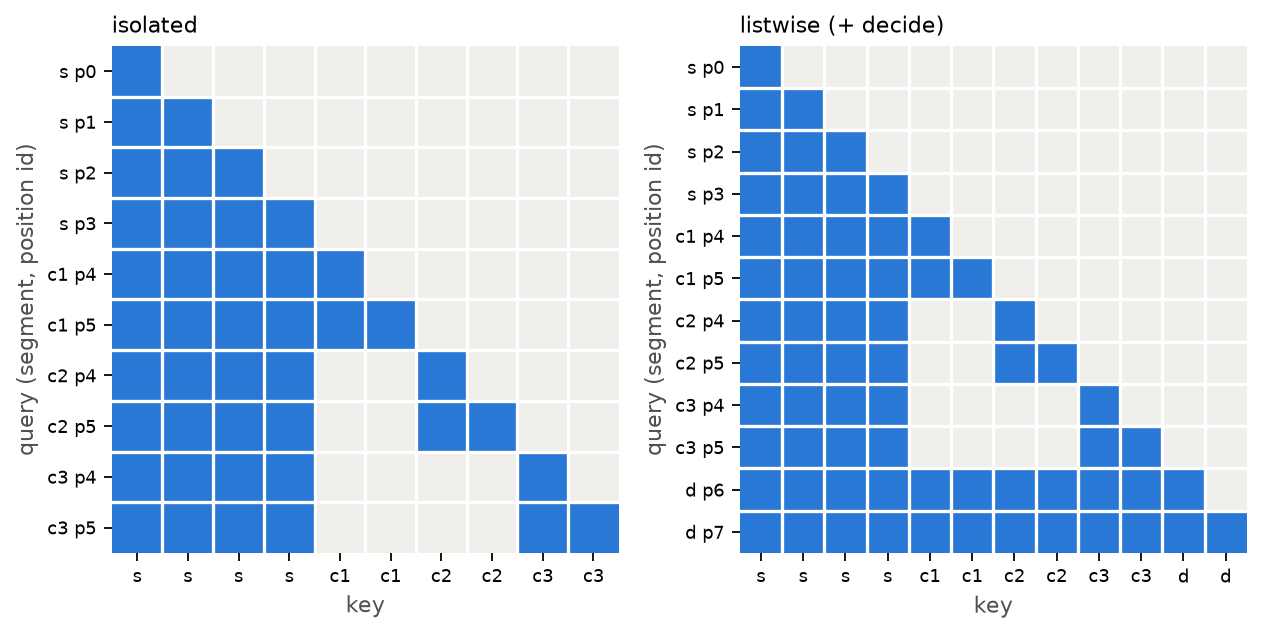
The masks exactly as jevrec.model.block_mask builds them for a 4-token state and three 2-token candidates. Every candidate restarts at position 4, so candidate i sees the same keys at the same positions as it would alone. That makes isolated the pointwise function, computed with one pass over the state.

Two practical notes. The mask trick needs a pure-attention backbone: linear-attention or SSM layers (for example Qwen3.5's Gated DeltaNet) ignore attention masks, which is why existing open reimplementations fall back to one row per candidate with a forked state cache on those models. And because the equivalence holds for the training forward pass too, you get the saving during training, not only at inference.

Results on MovieLens-1M

Qwen3-1.7B and Qwen3-8B, 1 epoch each, 2×B200 per run (about 23 and 75 minutes). 6,040 test users. "Auto @95%" is the share of requests you could decide automatically at 95% precision by thresholding confidence: the operating point calibrated decisions are for.

Rows without a tag are Qwen3-1.7B. Paired against SASRec on the same requests (McNemar; bootstrap 95% CI of the HR@1 difference): 1.7B −1.9 points, p=0.002, CI [−3.0, −0.8]; 8B +1.0 points, p=0.07, CI [−0.05, +2.1]. So 8B ties SASRec, it does not beat it.

Three observations.

Pointwise and isolated are the same model. Loading the isolated weights into the pointwise layout gives the same numbers to bf16 noise (0.6048 vs 0.6043), for ten times the tokens. The zero-shot rows agree too (0.084 vs 0.087).

Zero-shot quality depends heavily on scale. The 1.7B Yes/No readout is close to useless (0.087 vs 0.05 random), while 8B already reaches 0.282, above popularity. One epoch of LoRA on 48k decisions then closes the gap to SASRec for both. The 8B model is also the better decider: at 95% precision it can automate 27% of requests, against 23% for SASRec.

The listwise head is not idle but does not help. Its query projection grows from zero to norm 3.8 and it changes 8% of top-1 decisions, yet average HR@1, NLL and ECE are unchanged. With random negatives, "is this the next movie?" can be answered one candidate at a time. The natural objection is that the negatives are too easy, so we tested that next.

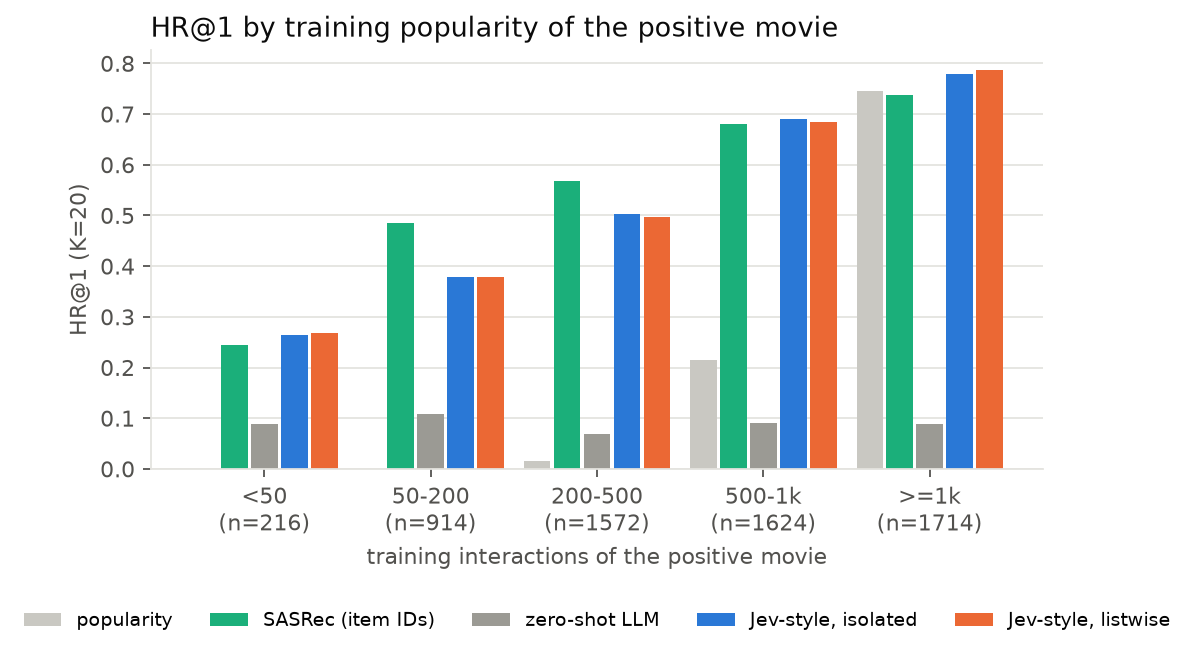
Where the gap to SASRec comes from. The LLM wins on the rarest positives (<50 training interactions, 0.264 vs 0.245) and on the head (≥500), and loses clearly in the 50–500 band, where ID embeddings have enough data to learn co-watch structure that titles and genres do not express.

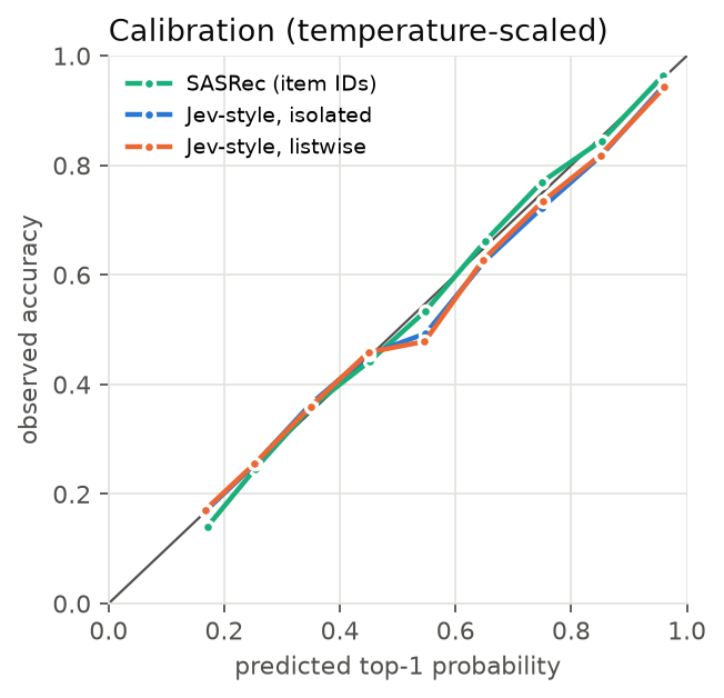
After temperature scaling (T≈1.2 for the LLM; raw ECE 0.071 → 0.023) both model families sit on the diagonal. Calibration is cheap for both, so it is no reason to prefer one over the other.

Harder negatives: removing the popularity shortcut

Uniform negatives are mostly obscure movies, so "pick the popular one" already gets 0.27 HR@1. We reran the 1.7B setup with the 19 negatives sampled in proportion to popularity (median negative popularity 562 instead of 107), for training and test alike.

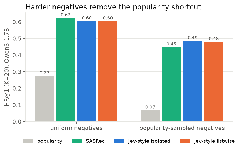
Popularity collapses to chance and SASRec loses 18 points; the LLM scorer loses 12 and now leads by 3.8 (McNemar p=1.5e-9, CI [+2.5, +5.0]). It also doubles the share of requests that can be automated at 95% precision.

Two conclusions. Part of SASRec's lead with uniform negatives was popularity, which ID embeddings encode very efficiently. And even when negatives are plausible, the listwise head does not help: it is 0.6 points worse at top-1 (p=0.03), with a hair better NLL. Scoring candidates independently against the user is enough here.

Downstream: a catalogue the model has never seen

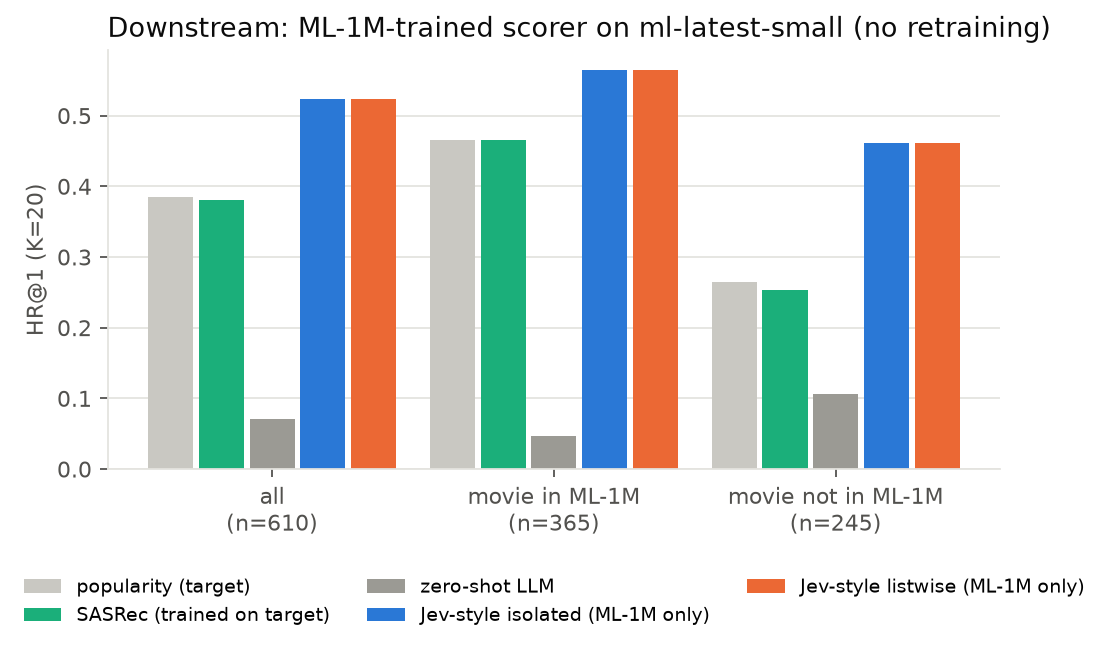
ML-1M stops in 2000. ml-latest-small is a 2018 MovieLens snapshot (610 users, 9.7k movies) with the same movie ids, so we can split its test positives into movies that exist in ML-1M and 245 that do not (228 of those were released in 2000 or later; the rest are older titles ML-1M never included). The LLM scorers are trained only on ML-1M and run unchanged. Popularity and SASRec get the easier deal: they are trained on ml-latest-small itself.

Rows without a tag are Qwen3-1.7B. Gains over SASRec: McNemar p=3e-8 (1.7B) and p=6e-16 (8B).

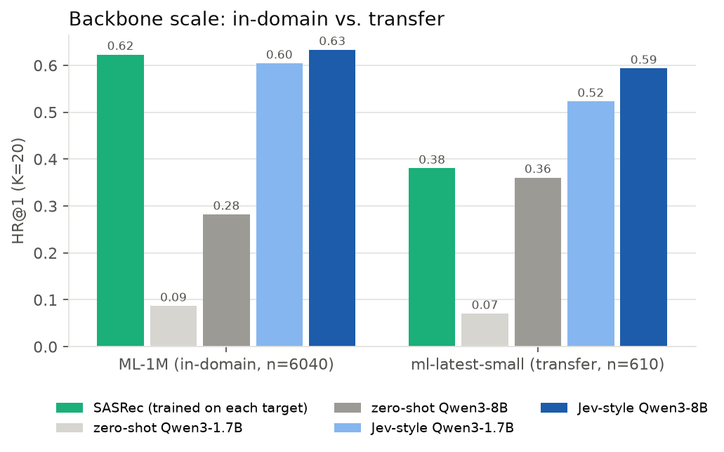
Moving from 1.7B to 8B adds 3 points in-domain and 7 points in transfer. The zero-shot readout gains even more (0.09 → 0.28 in-domain).

Cost

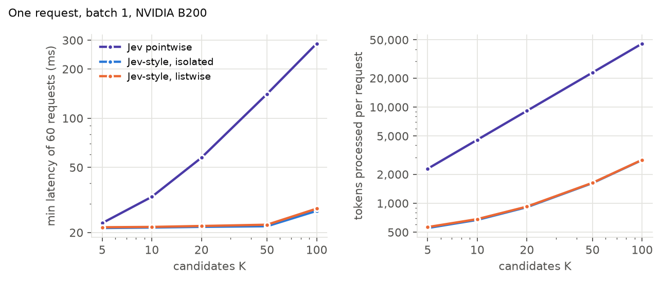
One request, batch 1, B200, Hugging Face eager + SDPA. The three modes share one backbone and are timed interleaved over 60 requests. We plot the minimum because the box is shared and requests stall intermittently by ~50 ms under host load (the medians are in the repo). Tokens grow as K·(state + candidate) for pointwise and as state + K·candidate for the masked modes. The masked modes stay at the ~21 ms launch floor of a 28-layer eager model up to K=50. Pointwise reaches 57 ms at K=20 and 286 ms at K=100, against 22 and 27 ms.

In recommender terms this is the familiar split between user-side and item-side computation. The masked layout computes the user once per request and each item once, the way a production ranker reuses user features across candidates, while keeping full cross-attention between each item and the user.

Takeaways

• If you build a Jev-style decision model on an attention backbone, use the block mask. It is the same function as the pointwise layout, and it cuts training and inference cost roughly by a factor of K for long states.
• As an in-domain ranker on a mature catalogue, an LLM scorer is competitive with, not better than, SASRec: 1.7B is 2 points behind, 8B ties. The case for it is elsewhere: calibrated typed outputs, no feature pipeline, and above all transfer to new items and new catalogues, where ID models start from zero.
• Listwise interaction is cheap (a zero-initialised bilinear term, 13 extra tokens) but did not pay off with either uniform or popularity-sampled negatives. Scoring each candidate against the user is enough here.

Reproduce

git clone https://github.com/wdlctc/jev-recommend && cd jev-recommend
pip install -e . && python -m pytest -q tests      # mask equivalence, CPU
GA=0,1 GB=2,3 bash scripts/run_all.sh              # train, zero-shot, baselines, latency
bash scripts/run_downstream.sh                     # ml-latest-small transfer
python scripts/analyze.py runs/q17b figures        # slices + figures